NFL Predictions
Introduction / Background
The cost of sports games is rising. The average cost of a football game in 2020 was ~ $105, which means, for those who can afford to attend a football game, there becomes a strong financial burden of attending multiple games. This puts a high level of importance on which game you choose to attend. Hopefully one that is high scoring? Close throughout? Keeps you on your toes until the very end?
Problem Definition
Machine learning can be used to predict which NFL games will be close in order to maximize fans’ entertainment based on their money.
Our goal is to run a model at the beginning of a season and to make confident recommendations to clients which of the games from the season are worth being the one game that year that they attend.
Data Collection
Datasets We used to create our dataset
Our dataset

Characteristics
- All regular season NFL games between 2003 and 2020.
- Each row represents a game between these dates.
- The columns include data about the score of each game, the quarterbacks for each team, the quarterbacks’ passer ratings from the previous season, each team’s win percentage for the previous season, and the total amount of points a team scored and had scored against them in a previous season.
- In addition, comparative columns were added, which include data such as the quarterbacks’ age difference, number of rookie quarterbacks per game, the quarterbacks’ combined passer ratings, each team’s previous season win percentage, each team’s previous season points scored, each team’s previous season points scored against, and the difference between the quarterbacks’ passer ratings.
Problems we encountered with data collection
- We originally wanted to use the total quarterback rating (QBR) instead of the passer rating because QBR incorporates much more information about how a quarterback contributes to winning than the passer rating does, which only takes passes into consideration. Unfortunately the QBR metric was not created until 2011 and was not used until 2012 so there was no data for any earlier seasons. We ultimately decided it was more important to have a larger dataset than to be able to use QBR.
- We had hoped to include more details about each game, such as each teams’ score at half time or every quarter; however, we found this data very difficult to come by and decided to exclude it.
- We could not find a single dataset that contained all of the data we wanted. For example, our dataset did not have previous season win percentages for each team. In order to add this to our original dataset, we found a different dataset which contained win percentages for each team during each season and then queried that dataset to add the previous season win percentages for both the home and away teams for each game.
Taking Care of Missing Features
In our dataset, we were missing some data for the quarterback passer ratings. This is because we used the passer ratings from the previous season for each quarterback, or the last season which they played in. Therefore if a quarterback was a rookie, meaning they did not play in the previous season or did not have any statistics from a previous season, then they did not have a passer rating.
We came up with a few ways to fill in the missing data.
Our first plan was to use the rookies’ passer ratings from their college careers. However, we found that this data was very difficult to find and not available for some of the rookies. In addition, we noticed that the passer ratings for college careers tended to be much higher than the passer ratings for the NFL so we felt this could skew our data.
After brainstorming a few other possibilities, we finally settled on taking the mean of all other passer ratings and using that average for the rookies. We felt this would give us the best results because, since we do not know how a rookie will perform in their first NFL season, we can assume that most rookies will perform around the average of all other quarterbacks in the NFL.
Methods
We first plan to use unsupervised learning to help reduce the load of the supervised models by attempting to find clusters within our independent variables. We will use the K-Means and DBSCAN techniques to do such clustering. We have considered two different methods of utilizing clustering:
- The first is to cluster the scores of each game and look to see if the clusters have other components in common, such as team, quarterback, etc. From there, we can categorize games in a way that is easier to use.
- The second option is to cluster based on the other independent variables, and we categorize each game as a “close game” or “not a close game” with a given threshold. We can then look at the clusters and see if there is a difference in the amount of close games within the various clusters.
From there, we will use the clusters we created in the first step, as well as our other data to create models that predict the outcome of the games. We will utilize a few different supervised learning techniques, such as logistic regression, SVM, and K Nearest Neighbor to predict the scores of games and the probability of a game being close. We will use unsupervised learning to help us better understand our data and our variables of interest.
Results and Discussion
Here we have presented two methods to approach the problem: unsupervised learning methods and supervised learning methods.
Unsupervised Learning
In order to cluster our data, we looked at using DBSCAN and K Means. We eventually settled on using K Means clustering because we found that our data was too dense for DBSCAN to provide useful clustering of our data. After running K Means and clustering around ‘score difference’ and ‘combined score’, we were given 6 clusters as shown below:

From this chart, we used the green cluster as the high scoring games that were close, light blue as the high scoring games that were not close, and the dark blue cluster as the low scoring games that were close. We chose these three clusters because we felt they represented the most interesting games to watch. In the future, we plan to look at the top ranking NFL games and see which clusters those games fall into.
We chose to cluster around score difference and combined score rather than the actual scores of each team. This is because we have defined an interesting game as a game that is high scoring, close, or both high scoring and close. We do not necessarily care about the actual score of each game, we just care about how high the scores are and the difference between the two scores.
Below is the clustering based on the home team and the away team.

From this chart, red represents a game where the home team scored much more than the away team, black represents a close, high scoring game, green represents a close, mid scoring game, light blue represents a game where the away teams scored much more than the home team, and dark blue represents a close, low scoring game. As one can see from the chart above, there is not a strong skew based on the home team and away team, which supports our idea that using the combined features (‘combined score’ and ‘score difference’ variables) does not lose much if any important information.
After clustering the data, we wanted to start looking into predictive models. We believed we had more variables than necessary, and were also worried about multicollinearity which could affect the results of our clustering, such as KNN. Given that we thought many of our variables were correlated, we wanted to use a principal component analysis to help reduce the variance within the factors.
In order to run a principal component analysis, we first needed to check that there was, indeed, correlation between the variables that we were using as our independent variables.
Below is the correlation chart. What we see is that there is not necessarily a strong correlation between most of the variables, though there is some correlation between the Combined PF, Combined PA, and Combined Win. For that reason, we originally decided not to pursue a Principal Component Analysis.
Correlation Chart

Data Split
We determined that because we will be predicting data about an entire year at a time, when we split the data, we want to split it by year not by individual game. For that reason, we split the data into 14 seasons for the training set, 2 seasons for the validating set, and 2 seasons for the testing set. For each of our models, we will train our models on the training set, we will tune our models using the validation set and select the best model based on the performance on the validation set. Once we have selected a model, we will retrain the model using the whole training and validation set of data, and then have a final unbiased estimate of our model accuracy by testing this new model on the testing set.
We defined the following years for our training years, our validating years, and our testing years:
- Training years: 2012, 2008, 2018, 2005, 2011, 2020, 2014, 2009, 2019, 2015, 2006, 2013, 2016, 2004
- Validating years: 2003, 2007
- Testing years: 2010, 2017
Supervised Learning
Our goal is to understand whether we can utilize information about the two teams in a game and past game outcomes, to predict which games would be good. For this purpose, whenever we discuss the accuracy of a model, we are talking specifically about the following: of the games recommended, how many are correct? In this instance, a model not recommending a good game is not a huge loss, but if we were to recommend a game to someone, we would want them to attend a good game.
Important Definitions
For the sake of our research, there are a few labels we feel it is important to define.
- Originally we defined a good, or interesting game, as a close and high scoring game. However, for the sake of our research, we decided to be more lenient with this definition and looked at close games, high scoring games, and close or high scoring games to be considered as good or interesting games.
- A close game is one whose teams are within 7 points of each other. This is because, generally, being within 7 points is considered a one possession game since a team can score that many points in one possession.
- A high scoring game is one where the combined score exceeds 42. This is because, at a minimum, there would need to be 6 scoring events for this to happen.
- Utilizing the above definitions, a close and high scoring game is one where the combined score exceeds 42 and the two teams are within 7 points of each other.
- A close or high scoring game is one where the combined score exceeds 42 or the two teams are within 7 points of each other.
- Lastly, as will be discussed below, a low scoring game is one where the combined score is less than 21.
Though these thresholds were determined utilizing our knowledge of football, the public perception of what is considered a good game, and the existing data we have, we did test whether different point cutoffs for a good game would provide better results. Our models’ performances did not improve with other cutoffs, so for the sake of simplicity, we do not include that research in this report.
Logistic Regression
We decided to attempt to use logistic regression to create a model that would help us predict a good game. For our logistic regression models, we tested two different sets of independent variables to predict three different variables: whether a game is close, whether a game is high scoring, and whether a game is close and/or high scoring. The reason we decided to test logistic regression with two different sets of independent variables is because, as previously mentioned, we were unsure if combining the team-specific variables (‘home team QBR’, ‘away team QBR, ‘home team win percent’, ‘away team win percent’) into combined variables (‘combined QBR’, ‘combined win percent’) would lose any valuable information that could help train our models.
Feature Set 1 - Team Specific Variables
This first logistic regression model is built using variables specific to the home team and the away team in each game. Specifically, we included previous win percentages of each team, previous points scored for each team, and previous points allowed for each team. Our hypothesis is that the win percent features might be useful for predicting the closeness of a game and the point aggregation features might be useful for predicting whether a game is high scoring.
Below are the features that we used for our first set of logistic regression models:
- home_team_previous_win_percent: the win rate (games won / games played) of the home team in the previous season
- away_team_previous_win_percent: the win rate (games won / games played) of the away team in the previous season
- home_team_previous_points_scored: the total points scored by the home team in the previous season
- home_team_previous_points_against: the total points scored against the home team in the previous season
- away_team_previous_points_scored: the total points scored by the away team in the previous season
- away_team_previous_points_against: the total points scored against the home team in the previous season
Close Game
Using these features, we first tried to create a model that would predict a close game. As a reminder, we described a close game as a game where the difference between the two scores was less than or equal to 7 points.


Unfortunately, this model did not prove to be very accurate at all, and was barely better at predicting a close game than choosing a game at random. Because of this, we experimented with a few different thresholds to define a close game (between 4 and 10), however, none of these improved our model.
High Scoring Game
Next, we attempted to use logistic regression to predict a high scoring game. As a reminder, we described a high scoring game as a game where the total score of the game was greater than or equal to 42 points.


This model did prove to be slightly more accurate than our first model; however, we determined that it was not accurate enough to provide us with any meaningful predictions. As we did with the previous model, we experimented with a few different thresholds to define a high scoring game (between 35 and 49), but these provided us with models that performed the same or worse than the original model.
Close OR High Scoring Game
After our models to predict a close game and a high scoring game failed, as a reminder, we decided to try to combine these two aspects to try to predict if a game is close or a game is high scoring.


Although this model seemed more promising at first because it had a decently high accuracy, we quickly realized a major flaw with this model. Although it was decently accurate at predicting games that were close or high scoring, it did not predict any games that were not close or high scoring.
Feature Set 2
The second set of features uses aggregated data across both teams. This means that, unlike in the first feature set where each feature had data for either the home team or away team, the features in this set contained averages or differences between the home and away team. Additionally, we included more general features about the teams (such as age difference of QB, the passer rating, etc). The reasoning behind this set was that specific team characteristics might play a role in determining the closeness or overall score of a game.
Below are the features that we used for our second set of logistic regression models:
- age_difference: the difference between the ages of the two quarterbacks
- rookies: the number of rookie quarterbacks in the game
- combined_passer: the average of the two quarterbacks’ passer ratings
- combined_win: the average of the two teams’ win percentages from the previous season
- combined_PF: the average number of points scored by the two teams from the previous season
- combined_PA: the average number of points scored against the two teams from the previous season
- passer_difference: the difference between the two quarterbacks’ passer ratings
- PF_difference: the difference between the number of points scored by the two teams from the previous season
- PA_difference: the difference between the number of points scored against the two teams from the previous season
Close Game
Using this new set of features, we wanted to create a model that would predict a close game.


Unfortunately, this model performed very similarly to its counterpart using the first set of features. Since these models performed about the same, we determined that there was no point testing other thresholds for a close, since it would result in either the model performing the same or worse.
High Scoring Game
Next, we attempted to create a model that would predict a high scoring game with our new set of features.


This model also performed similarly to its counterpart using the first set of features. Although it was also more accurate than the model to predict a close game, it did not have a high enough accuracy to provide us with a useful predictive model.
Close AND High Scoring Game
Unlike our approach with our first set of features, since our more lenient definition of a good game was not providing us with the results we had hoped, we decided to try modeling the logistic regression around the games that are of the most interest: high scoring games that are also close. Given we’re now trying to recommend games that are close AND high scoring, we hoped that it would avoid the issue of predicting too many games in this category.


Unfortunately, this model ended up having a similar problem to the model that tried to predict if a game was close or high scoring. This model failed to predict any games that were close and high scoring.
Best Threshold
Since these models did not prove to be very successful, we also tried different thresholds for deciding the predicted label within logistic regression (the default was 0.5) to see if this would increase the accuracy at all. Unfortunately, this did not improve the accuracy significantly since the optimal threshold turned out to be very close to 0.5.

Additional Models
Since we were unable to obtain any useful models for predicting what we considered to be interesting games (close games, high scoring games, or both), we decided to see if we could possibly predict an uninteresting game. If we were able to create a model that could predict an uninteresting game, we could at least recommend games that people should not attend. Although this would not fulfill our original goal, it would at least provide us with a useful predictive model.
In order to test this, we defined an uninteresting game as a game where the difference between the scores was large or a game where the total score was low. We attempted to predict games with a large score difference, very low scoring games, and games that fell into both of these categories. Unfortunately, these models also provided a very low classification accuracy. One of our hypotheses for why this occurred is due to the fact that very few games in our dataset fall into these categories, which means it may be harder for models to find differences.
Logistic Regression Conclusion
After trying many combinations of features and labels as well as different predicted label thresholds, we have decided that a logistic regression model is not optimal for predicting certain aspects of football games. We were not able to use this model to accurately predict how interesting (where “interesting” refers to the dependent variables discussed above) a game might be.
Something we came across was that many of our logistic regression models would either predict every game as the classification of interest or none of the games. A potential reason for this could be because our data did not have enough information to predict a label or there was such a disproportionate amount of data in one class that there was not enough variability in the data to properly train the model. Based on our data, we believe that the latter was most likely the cause. We believe that the reason that this error occurred in our model was due to the fact that we did not have enough data with enough variability in the independent variables for our model to accurately predict the classification of games.
SVM
In the Support Vector Machine model, we devised four classifiers and two of them demonstrated relatively good accuracy scores around 0.8.
In this model, the independent variables used are score1, score2, age_difference, combined_passer, combined_win, combined_PF, combined_PA, passer_difference, PF_difference, and PA_difference.
In order to classify all the games, we devised four classifiers: 1) The score between two teams is close OR the combined score is high 2) The score between two teams is close 3) The score between two teams is close AND the combined score is high 4) The score between two teams is close AND the combined score is low
When choosing the threshold in order to measure what a close scoring game is and what a high scoring game is, we applied the same threshold used in Logistics Regression. That is, any game that has a combined score over 42 points is considered a high score game, and any game that has a score difference less than 7 is considered a close game.
Classifier 1
Initially, we were searching for a good game, a game with classifier 1: The score between two teams is close OR the combined score is high. After running the model, both the accuracy score and the precision score were good (shown in classification report below), but this classifier gave us way too many recommendations (452 predicted good games). Although the recommendations were valid and very likely to be good games, the classifier did not effectively narrow down good choices for the audience.

Classifier 2
Next, we narrowed down the classifier to just predicting a close game with classifier 2. Ideally, this classifier would help us bring the number of recommended games down..
The number of recommended games in this classifier was 208 (shown below), but the accuracy score went down to 0.54 and the precision score went down to exactly 0.5. In addition, if the game was just a close game, it does not necessarily prove that the game is a good game. Therefore, we decided to add in another two conditions for further exploration.


Classifier 3
The next classifier that we used was classifier 3, which predicted if a game was close and high scoring. The performance report is shown below.


As you can see, this classifier does give a better accuracy score of 0.74 and effectively narrows down the games to 41, but the precision in determining whether this is a good game is too low, at only 0.49. Therefore, this classifier is not very reliable.
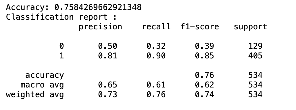
Classifier 4
Lastly, we looked at the last classifier, classifier 4, which predicted if a game was close AND low scoring. This classifier gave us the highest accuracy out of the four tested, with an accuracy of 81%.


This classifier provided us with a smaller recommendation subgroup, but it had the same problem as classifier 3, low precision on predicting positive labels.
SVM Summary
In order to recommend games, we need a model that gives us a good accuracy score, but does not recommend too many games. The only way to narrow down the recommendation number is to strictly filter good games with related conditions. When we applied such a mechanism in classifiers 3 and 4, the use of SVM provided us with a decently high accuracy score when classifying games; however, in terms of precision score when testing the positive label, neither of the classifiers produced an ideal model. Therefore, in the end, we were not able to find a SVM classifier that satisfies our requirements. For future research, we could look into the different combinations of our independent variables in order to increase precision score for positive labels.
KNN
After attempting to utilize SVM and Logistic regression, we decided we wanted to try KNN as a means of answering the question; can we utilize information about the two teams of a game, and past game outcomes, to predict which games would be good.
Similar to Logistic regression and SVM, in order to do this, there were a few different classifications of good games that we initially decided to consider: a game that was close, a game that was high scoring, and a game that was close and high scoring.
One of the things in KNN that we had to consider when determining the best K is that we wanted a high level of accuracy, but we also cared about how many games were being recommended. If we set the threshold of a good game such that our model can correctly recommend 150 games that are at least just fine, that does not provide enough guidance to be of use to a possible stakeholder. Additionally, if our model is set up in a way that it only recommends three games with the validation set, even if it perfectly classifies those three games, there is a higher possibility of this model being overfit and thus being unreliable to utilize as a means of prediction outside of our validation set.
Close Game
To look into whether or not we can predict a close game using KNN, we utilized the training dataset, and looked into what threshold of K provided us with the best accuracy on the validation data. Taking into consideration what was mentioned above, the range in K provided an accuracy of anywhere from 42% to 49% and classified anywhere from 158 to 248 games as being close. Our best model was with a K of 45.

Given that 246 of the total 534 games in our validation set were considered close, a model whose accuracy rate is less than 50% provides us no better odds of selecting a close game than if we randomly selected one ourselves.
Close and High Scoring
Similarly, looking at games whose combined score were greater than or equal to 42 did not provide us with any helpful recommendations. Thus we looked at games that were both close and high scoring. Within the validation set of 534 games, 114 games fell into this category. Again, we tested different values of K, taking into consideration wanting a higher percentage of accuracy, while still keeping the right balance of the number of recommendations.
When looking at different values of K, the models’ accuracies ranged from 22% to 50%, and the number of games recommended ranged from 3 to 118. Below is the graph of the percent accuracy and the number of games recommended. With this data, we went for the highest number of recommendations that provided the highest accuracy percentage, so we went with a K of 27 (as shown below).

The model classified eight games from the validation set as being close and high scoring, when in reality, only four of them were close and high scoring.

Although KNN was not providing the most promising results, we decided to try to classify games as being close OR high, utilizing the existing thresholds. Unfortunately, 399 of the games fell into that category, which meant, even with a 75% accuracy rate, it was not any better than randomly choosing a game (since 399 / 534 > 75%)
Since trying different cutoffs for a good game did not provide us with better results, we decided to return to our 50% accuracy model. We were curious how bad the misclassifications were. Of the four games that were wrongly recommended, three were very high scoring but not so close, and one was close but not that highest scoring. So we decided to look into this model a bit more. We decided to try to change the thresholds of a close game and high scoring, but also, potentially try to change the way that the KNN function rounds.

With this in mind, we tried different thresholds, retaining the goal of not wanting too many predictions, but also not wanting too few, and trying to maximize the percent of true predictions. We realized that if we adjusted the rounding threshold for the KNN prediction output to .49, we would actually have a higher response rate:

With a K of 27 and a threshold of .49, our best KNN model classified 9 of the games from the validation set as good games, with 5 of them being high scoring and close, and the other 4 being high scoring or close.
However, since numerous of our models did not perform well, we were curious about whether there were better inputs for our model.
PCA
Although we decided that PCA may not be an effective modeling strategy, given our inability to develop another effective model, the knowledge KNN generally works better with fewer inputs, and that we know that there are a few correlated variables within our data, we decided to try PCA to see whether dimension reduction could help fine tune the KNN model.
After looking at the explained variance by dimensions, there was not a clear elbow, so we tried the KNN using two of the principal components and three. Both of these models performed worse than the initial model. We realized that our possible issue was underfitting not overfitting, so PCA was not helpful.

KNN Revisited
After attempting to utilize PCA to improve our KNN model, we decided there were a few other types of KNN models we wanted to train. First, instead of using our classification of a good game, we tried to use the clusters from our KMeans. Secondly, similar to logistic regression and SVM, we tried to train our model to classify bad games instead of good games (low scoring or blow outs) as means of recommending what games not to go to. Unfortunately, none of these models provided us any reliable method of predicting.
KNN Summary
We decided that maybe KNN was not the right approach to ultimately predict good games. That being said, we feel comfortable that our KNN model that suggested nine games showed some promise of being a useful model since none of these games it predicted were considered bad games. However, there is a chance that this is due to overfitting, rather than being a successful model.
Conclusion
Despite trying KNN, SVM, and Logistic regression, we were unable to come up with a model that can accurately predict at the beginning of a season which games are going to be close and high scoring. However, we did have a KNN model that, by looking at close and high scoring games with a K of 27 and a threshold of .49, could provide some helpful information. By retraining this model with the full training and validation dataset and testing using our testing dataset, we were able to obtain 12 game recommendations. Only 2 of these games actually fall into the category of close AND high scoring, but 8 of them fall under the category of close OR high scoring. This means that, given 46% percent of games in the testing dataset are close, 57% percent are high scoring, and 26% percent are close and high scoring, even utilizing our best model, you’re probably better just deciding on a game on your own.


Analysis
Overall, we realize that our approach to solving our problem was flawed in some way because we were unable to obtain a model that could accurately predict interesting NFL games. After testing numerous models and in general getting similar results, we believe that the issue ultimately lies within our data, rather than with our approach.
One potential explanation is that we did not use enough data. When collecting our data, we only considered games from 2002 and 2020. The reason that we settled on these years was due to the fact that 2002 was the earliest year that contained data for all of the categories we considered. We decided to do this because we felt it was more important to have more categories of data rather than more years of data. However, it is very possible that this was a mistake and we should have sacrificed having more categories of data for more years of data.
Another possibility is that we made too many assumptions as to what contributes to the outcome of a game. In our data, we felt that the aspects that would affect the outcome of a game the most were the following: the quarterback (his passer rating, if he was a rookie, his age) and the performance of a team in the previous season (the win percentage, the number of points score for and against). However, it is very possible that these aspects have a much lower impact on a game than we assumed. For example, just because a team did well in a previous season does not necessarily mean they will do well in the current season. Some of the top players may leave the team or the coach may change. In addition, it is possible that the quarterback is less relevant to the outcome than we assumed. Although the quarterback is often seen as the most important player in the game, it is possible that having a strong defense or a good coach may have a larger impact.
In conclusion, we believe that our shortcomings in this project were likely caused by our data rather than our methods. More research and further study could eventually allow us to yield a successful model to solve our problem of predicting interesting NFL games at the beginning of a season to recommend for fans to attend.
Process Learnings
Through this work, we learned that not all models will necessarily work for every dataset. For example, we thought DBSCAN might be useful, but given the density of our data, DBSCAN generally just created one giant cluster with outliers rather than useful clusters.
We also learned that we need to do more work in the beginning to understand our variables, understand the multicollinearity between our variables, and find ways to perform variable selection that reduces some of this.
Suggestions for Future Study
As discussed above, we believe that the flaw in our project resulted from our data. Because of this, we feel that there are numerous areas for future study that could help us create a useful model to solve our problem.
Originally, we had wanted to include data with the different scores by quarter in order to add more variability to the games. However, we were unable to find a data set that included this data. Because of this, we decided to exclude this from our dataset because we knew collecting this data would be extremely time consuming. In the future, it may be beneficial to spend the time to collect this data.
Another form of data we felt might be interesting would be to look at more dynamic variables, such as how teams performed against one another historically, or what is considered as a rivalry game or not. Although it may seem that this data may not have an impact on the outcome of a game, many teams tend to “choke” or perform worse when they are playing against a rival or a team that they have lost to numerous times in the past.
Furthermore, the only dimensionality reduction process that we attempted was PCA. In the future, it may be beneficial to run other similar processes, maybe variable selection processes such as Lasso or Elastic Net in order to possibly limit the collinearity.
And finally, though we attempted to obtain data from as far back in time as we could, we were unable to do so as different public data sources started their data collection from a variety of different years. Due to this, we had several holes in different aspects of our data for the very early years and decided to omit them from our dataset due to time constraints. In the future, for more data on game history, it would be helpful to take the time to fill in the gaps in the earlier years.